This tutorial delineates a How-To for detecting distinct groups within a multivariate dataset – a much needed task albeit with numerous open issues and methodological pitfalls.

The procedures described here follow those described and applied in the (currently revised) manuscript:

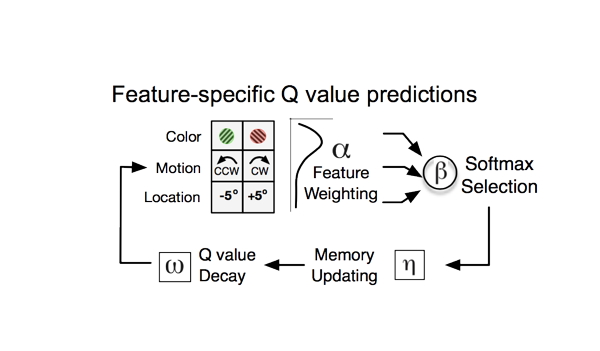
• Goulas A, Westendorff S, Everling S, Womelsdorf T (under review) Functional segregation of cells coding for valuation, choice and chosen features in macaque anterior cingulate and prefrontal cortex.

Specifically, we are making use of a class of algorithms called module detection algorithms. This tutorial is not meant to offer an in-depth presentation of the issues around this class of algorithms, but enable interested users to perform the analysis. For more details the interested reader can refer to the following papers (referred to in detail in the above manuscript): Newman, 2006; Rubinov and Sporns, 2011; Good et al., 2010.

All the analysis described can be performed in MATLAB and the following freely available toolboxes:

• Fathom Toolbox (Jones, 2014)
• Brain Connectivity Toolbox (Rubinov and Sporns, 2010)

Place the folders of the above toolboxes in your Matlab path in order to be able to use the .m functions mentioned below.

Module detection algorithms operate on data represented as graphs: a collection of nodes (N) and edges (E) between them denoting the “relation” of the nodes. Thus, a NxN graph contains all the information on the relations between all pairs of nodes. Note that the graph can be directed or undirected, i.e. The latter entailing that the upper and lower triangular parts are identical. The methods described here concern undirected graphs, but module detection algorithms work on directed ones as well.

In order to obtain the NxN graph, we have to capture all pairwise relations of the items of a multivariate dataset NxM. In other words we have to measure the similarity between the items. There are many similarity measures with different value ranges (positive and negative), capturing a different aspect of the relation between two items in the dataset. Thus, careful choice of the similarity measure is important is important. In our dataset D, we choose Pearson’s correlation coefficient as a similarity measure. You can use for similarity measures the function pdist.m. With the calculation of all pairwise similarities we obtain the NxN similarity matrix functioning as the graph Sim to be analyzed: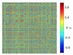

Note that since we used Pearson’s correlation we have both positive and negative values. This is not a problem since module detection algorithm can handle grahs with negative values. Note as well that there is not need to discard any entries by thresholding the graph (apart from ensuring that the diagonal contains only 0s) since the methods described here can also handle fully connected graphs.

We can examine if the dataset can be partitioned in modules with the following function:

>>[Ci Q] = modularity_louvain_und_sign(Sim,'sta');

where Ci is the module index with unique integers marking the entries belonging to the same module and Q the modularity value. Note that the argument ‘sta’ indicates how the positive and negative contributions for the modularity are combined (for other options and details see Rubinov and Sporns, 2011). The value Q is the value that the algorithm is trying to maximize and among many ways the aforementioned function implements the Louvain algorithm (Blondel et al. 2008) for signed graphs. Thus, the higher the Q value the more “modular” well partitioned the dataset is (maximum Q→1). If the graph does not contain negative weights, this function can be used instead:

>>[Ci Q]=modularity_louvain_und(Sim);

The functions described below concern graphs also containing negative values but corresponding functions for graphs without negative entries are also available as part of the Brain Connectivity Toolbox.

Optionally, we can fine tune the partition with the following functions that performs an opertion similar to a Kernighan-Lin fine-tuning:

>>[Ci Q]=modularity_finetune_und_sign(Sim,'sta',Ci);

Importantly, the algorithm will return potentially different solutions each time with very similar Q values something known as degeneracy of the modularity. Therefore, many runs should be applied. Instead of choosing only one solution out of many based on e.g. the one exhibiting the highest modularity, it is advisable to try to combine all the solutions to form a consensus partition with e.g. the following function:

>>Ci_Consensus = consensus_und(d,tau,reps);

where d is a NxN matrix with entry i,j denoting the co-occurrence of the respective nodes in the same module in the solutions generated from the module detection algorithm, tau a threshold applied at each step to the matrix d and reps the number of repetitions of the module detection algorithm (see Lancichinetti and Fortunato, 2012 for details). For instance if the co-occurence matrix has entries ranging in [0, 1] (0=never in the same module 1=always in the same module), we could run the consensus function as follows:

>>Ci_Consensus = consensus_und(d, 0.5, 100);

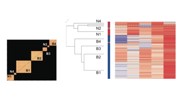
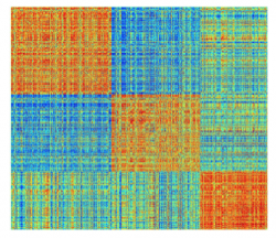
The Nx1 vector Ci_Consensus contains the integers denoting the nodes deemed to be in the same consensus module partition. For instaance if the modularity algorithm detected 3 groups, the following command will visualize the similarity matrix ordered to reveal the detected modules:

>>imagesc(Sim(vertcat(find(Ci==1),find(Ci==2),find(Ci==3)),vertcat(find(Ci==1),find(Ci==2),find(Ci==3))));

It is important to note that the module detection algorithm will always return a solution Ci and a modularity value Q even when applied to a random dataset! Therefore, it is crucial to assess if the solution obtained from the original data is “surprising” when compared on what to be expected “by chance”.

A basic way to generate a null model is to shuffle the edges of the graph (positive and negative with equal rate):

>>R=null_model_und_sign(Sim, 10);

By feeding the null matrix R in all the functions that were used to analyze the original matrix many times we can obtain a null distribution of the Q values and compute the corresponding p-values and z-score.

Many null hypothesis scenarios can be valid for various cases, each one of them aiming at exploiting specific idiosyncrasies of the data and/or the similarity metric used. Therefore it is advisable to construct null models that control for specific aspects of the data analysis. For instance, in the case of a NxM multidimensional dataset, we can permute the dimensions of each data point N and subsequently compute the similarity matrix. This creates a “null” relation that exists among two data points in the M dimensional space. Obtaining null matrices from such a procedure again leads to the estimation of the null distribution of the Q values and allowing the computation of the corresponding p-values and z-score.

Given a partitioning of N datapoints of a NxM multivariate dataset into K groups, e.g. by using the aforementioned module detection algorithm, it is instructive to unveil the most prominent dimensions contributing to the “separability” of the groups. One way to answer such a question is through the use of Canonical Discriminant Analysis (CDA). CDA is similar to Principal Component Analysis but instead of seeking to explain most of the variance between the datapoints, it focuses on between groups variance (see e.g. Legendre and Legendre, 1998 for more details). We can perform CDA with the following function:

>> [result]= f_cda(D,Ci_Consensus,2,1000,1,0) ;

Note that the struct “result” contains also many useful statistics such as Wilks’ lambda and trace stats and also their respective p-values.

>>f_cdaPlot(result,0,0,0,0,1,0,{'Offer','Shift','Attention','Rotation','Choice','Reward','ITI'},'tex');

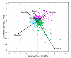
The above figure projects the M dimensional data in the 2D space spanned by the first canonical axis. Note that since we only have 3 groups the 2 canonical axis explain in total 100% of the variance. Note the good separability of the groups and the prominent role of the dimensions/features Sustain Choice and ITI and evaluate for the separability of the 3 groups. In the aforementioned example (grouping of neurons based on their functional temporal profile across 7 dimensions:’Offer’,’Shift’,’Attention’,’Rotation’,’Choice’,’Reward’,’ITI’) we have 7 dimensions but other datasets of course can have an, in theory, arbitrary number M of dimensions/features.

Blondel VD, Guillaume JL, E L (2008) Fast unfolding of communities in large networks. J Stat Mech P10008.

Good BH, De Montjoye YA, Clauset A (2010) The performance of modularity maximization in practical contexts. Phys Rev E 81:046106.

Jones DL (2014) Fathom Toolbox for Matlab: software for multivariate ecological and oceanographic data analysis. College of Marine Science, University of South Florida, St. Petersburg, FL, USA. Available from: http://www.marine.usf.edu/user/djones

Legendre P, Legendre L (1998) Numerical Ecology 2nd Edition: Elsevier.

Newman ME (2006) Modularity and community structure in networks. Proc Natl Acad Sci U S A 103:8577-8582.

Rubinov M, Sporns O (2010) Complex network measures of brain connectivity: uses and interpretations. NeuroImage 52:1059-1069.

Rubinov M, Sporns O (2011) Weight-conserving characterization of complex functional brain networks. NeuroImage 56:2068-2079.