This site is under construction. It will outline the analysis sequences needed for co-registering, 3D rendering + visualizing, and area labeling ECoG strip and grid data.

The procedures described here are applied in the manuscript:

• Micheli C, Kaping D, Westendorff S, Valiante T, Womelsdorf T Inferior-frontal cortex phase synchronizes with the temporal-parietal junction prior to successful change detection.

The procedures shown here have the goal to represent electrocorticography electrodes in a standard MNI three-dimensional space (colored AAL labels in the right panel). Eventually, the result of electrodes’ reconstruction leads to representations such as these:

This tutorial provides a step-by-step guide to achieve the reconstruction and the visualization of ECoG electrodes in the MNI space.

Pre-requisites are :

1. Have a pre-surgical MRI anatomical scan of the subject
2. Have a post-implant CT scan of the subject in which the electrodes are visible (the brain might ‘sag in’, and this requires additional processing to project the electrodes back on the pre-surgical MR scan cortex surface)
3. Know the labels of the electrode and how they relate to the electrophys recordings. It is STRONGLY ADVISED to mark the electrodes (see manual marking step later on) with the same order as in the ECoG recordings.

This is the first step in the whole procedure and requires Matlab software and the installation of a well-known free open-source software for MRI and fMRI analyses (recently also EEG and MEG analyses) called Statistical Parametric Mapping (SPM). You can download it here: SPM
Currently SPM12 version is available, but we use SPM8 in this tutorial to avoid compatibility and stability issues with the tutorial results.
Another software that we use extensively is FieldTrip (also open-source and freely downlodable from the link). Please read the instructions in the sw’s main page to receive automatic updates (the toolbox is upgraded daily/weekly with new functions).
After installation and after adding the toolboxes to your Matlab path, from within the workspace do:

mri = ft_read_mri('name_of_the_first_mr_file');
ct = ft_read_mri('name_of_the_first_ct_file');

to generate the volumetric variables for the MRI and the CT scan volumes. Partial information from the headers is also incorporated in the mri and ct structures (FieldTrip syntax is adopted).
A volumetric image (or simply ‘volume’) is a set of gray-scale intensity numbers ordered along 3 cartesian directions (x,y,z), originally called ‘voxel space’, which represents the adimensional space of the digitized image information, or in other words, the space of the acquired slices, stacked one upon each other. Normally the sampling of the physical scan space is not homogeneous in all 3 dimensions; in fact, more commonly the ‘slices’ are sampled homogeneously (e.g. x and y), but the slice distance is coarser (z axis).
To correct for this non homogeneity (for reasons that will become clear later), we apply a ‘reslicing’, which has the consequence to render the volumetric elements (voxels) homogeneous in the 3 cartesian directions (x,y,z). We do it like this:

% example for ct only (same for mr)
[tmpmin] = ft_warp_apply(ct.transform,[1 1 1]);
[tmpmax] = ft_warp_apply(ct.transform,ct.dim);
tmp = sort([tmpmin;tmpmax],1);
xyzmin = tmp(1,:);
xyzmax = tmp(2,:);
cfg = [];
cfg.resolution = 0.4;
cfg.xrange = [xyzmin(1) xyzmax(1)];
cfg.yrange = [xyzmin(2) xyzmax(2)];
cfg.zrange = [xyzmin(3) xyzmax(3)];
ct_r = ft_volumereslice(cfg,ct);

After this, we can save the resliced image on disk (with FieldTrip/SPM), start the spm8 GUI and visualize the homogeneous volumes:

Note that the head in two modalities “looks” in opposite directions. This is due to scan conventions (acquisition order of voxels along the three main directions). In the next step we will see how to realign and fine-coregister the two volumes with each other.

Note that the CT is the ‘source’ image and MRI is the ‘target’ in the SPM interactive window (left).

After coregistration the CT is expressed in MRI coordinates. The next step is to use MRCT toolbox to manually mark the electrodes (left pic), for each slice (select the projection which best suits this task). The toolbox also allows for a labelling of the electrodes (assignment of a number to the electrode position). Normally the label-number (right) corresponds to the order in which the electrodes are saved in the electrophysiology recordings.

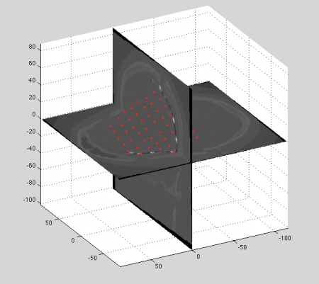
Finally, the marked electrodes (red dots) look like this compared to two perpendicular CT slices (in MR coordinates)