


The Waveform Analysis toolbox for cell-type identification
The Waveform Analysis (MATLAB / GNU Octave) toolbox classifies broad vs narrow spiking neurons based on the characteristics of extracellularly recorded action potential (AP) waveforms. This toolbox was developed and is maintained by Salva Ardid PhD.You can download the matlab code here matlab-files (zipped).
The code reproduces Figure 1 of the paper:
-
Ardid S., Vinck M., Kaping D., Marquez S., Everling S., Womelsdorf T. (2015) Mapping of functionally characterized cell classes onto canonical circuit operations in primate prefrontal cortex. Journal of Neuroscience. [pdf link to come soon, for pre-print please email us].
This toolbox is free but copyrighted by Salva Ardid, and distributed under the terms of the GNU General Public Licence as published by the Free Software Foundation (version 3). Should you find the toolbox interesting, please try it in your data. Just ensure that any publication using this code properly cites the original manuscript and links to this repository: – Ardid, Vinck, Kaping, Marquez, Everling, Womelsdorf (2015) Mapping of functionally characterized cell classes onto canonical circuit operations in primate prefrontal cortex. J. Neurosci. In Press.
Copyright (C) 2014-2015, Salva Ardid.
Intro
The basics of the method are similar to previous attempts, but it is improved with respect to others in at least some of the following aspects: Bimodality of waveforms was enhanced and thus better discriminated by including, in addition to the peak to trough duration, the time of repolarization (Fig. 1A and 1B in the paper). We combined the two measures by means of a principal component analysis (PCA). Cell-type discrimination was then based on the first component of the PCA (Fig. 1B and 1D in the paper). Non-unimodal distribution of waveform measures are typically analyzed using the Hartigan’s Dip test. However, sensitivity in rejecting unimodality is enhanced by using its calibrated version instead, especially when a different proportion exists between the two modes, as it is the case for narrow and broad spiking cells (Fig. 1B and 1C in the paper). Unimodality rejection in Hartigan’s Dip test (as well as in its calibrated version) is sensitive to discontinuities in the distribution. For waveform measures it is then essential to previously diminish by non-linear (e.g. cubic spline) interpolation the discontinuities that are artificially introduced by the sampling frequency of waveforms. Tutorial for the Waveform Analysis Repository The main script to execute the code is main_wf_analysis.m. It first loads the original data wForig.mat that contains an structure of the same name wForig with the following fields:
-
Unordered List ItemW: averaged AP waveforms (1138×52: number of independent recordings including single and multi-units, times the number of samples of their waveform).
-
Unordered List ItemX: time steps of the samples.
-
Unordered List Itemisolationquality: 0-3 categorical code that describes the likelihood that the avg. waveform corresponds to a single unit.
-
Unordered List ItemisolationqualityInfo: meaning of the corresponding numbers; 1) multiunit, 2) mostly single unit, 3) highly isolated single unit, 0) not specified.
-
Unordered List Itemdatasetname and spikechannel: self-explanatory; identifiers of the datasetname and spikechannel from where the averaged AP waveform was processed.
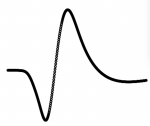
A typical AP waveform looks like this:
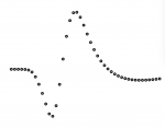
Cubic spline interpolation of AP waveforms
A cubicly interpolated (spline) AP waveform looks like this:
Not interpolated AP waveform
Cubic spline interpolation of AP waveforms
A cubicly interpolated (spline) AP waveform looks like this: Interpolated AP waveform The waveformPreprocessing function is called with configuration parameters cfg: troughalign: whether an alignment for all AP waveforms at their minimum value (trough) should be done (1 by default). interpn: interpolation factor (>1; 10 by default). interptype: type of interpolation to be used (spline by default – note that no benefit would be obtained from linear interpolation, see point 3 of the Intro). normalize: whether to normalize AP waveforms in [-1,1] (1 by default). fsample: sampling frequency (40kHz in this case). In addition to the configuration parameters, the function needs the avg waveforms W and the isolationquality from the wForig structure (note that only highly isolated single cells are considered):
[W, X, par, parName] = waveformPreprocessing(wForig.W,cfg,wForig.isolationquality);
The waveformPreprocessing function returns the interpolated waveforms W, the new time steps of the samples X, and the computation of distinct measurements from the AP waveform (par; and parName that describes those):
-
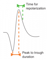
Unordered List Itempar(:,1) contains the peak to trough duration: time interval from the minimum W to its maximum.
-
par(:,2) contains the amplitude of peak before depolarization (currently not used).
-
par(:,3) contains the time for repolarization: time interval from the maximum W to the 25% of the peak to trough amplitude during repolarization
All relevant variables are then included in the wFpreprocessed structure
Separation of cell types according to AP waveforms
Only the peak to trough duration and the time for repolarization are considered, and only for highly isolated single cells. From to the two, the analysis is applied to the first component (PC1) from the principal component analysis (PCA). For comparison, the code is also applied to them individually, but I will focus here only on PC1. The waveformSeparation function the is called as follows:
[dipPCA,pdipPCA,xlPCA,xuPCA,ind_narPCA,ind_broPCA,ind_fuzPCA,aicPCA_1,aicPCA_2,bicPCA_1,bicPCA_2] = waveformSeparation(Xpca1stcomp,'PCA1stComp','First component of the PCA',Xlim,mu,sigma,pcomponents,FIGSDIR);
The input arguments are:
-
Ordered List ItemXpca1stcomp: the measure of the AP waveform, PC1 in this case.
-
Ordered List Item’PCA1stComp’: short explanatory label for the measure.
-
Ordered List Item’First component of the PCA’: long explanatory label for the measure.
-
Ordered List ItemXlim: range of the measure distribution.
-
Ordered List Itemmu: estimate of the mean of each component in the 2-Gaussian fit.
-
Ordered List Itemsigma: estimate of the covariance matrix of each component in the 2-Gaussian fit.
-
Ordered List Itempcomponents: estimate of the mixing proportions of each component in the 2-Gaussian fit.
-
Ordered List ItemFIGSDIR: refers to the subfolder where to save the resulting plots.
The output arguments refer to:
-
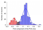
Ordered List ItemCalibrated Hartigans’ dip test: [dipPCA,pdipPCA,xlPCA,xuPCA]. pdipPCA < 0.05 discards unimodality.
-
Ordered List ItemClassification of cells into three groups: narrow (ind_narPCA), broad (ind_broPCA) and unclassified or in-between neurons (ind_fuzPCA) according to a 2-Gaussian model. According to that model, unclassified neurons are those for which the likelihood to be considered narrow is not larger than 10 times the likelihood to be broad, and vice versa.
-
Ordered List ItemAkaike’s and Bayesian information criteria for the 1-Gaussian vs 2-Gaussian models: [aicPCA_1,aicPCA_2,bicPCA_1,bicPCA_2]. Within a criterion, the lowest value is considered best.
The waveformSeparation function also creates two plots that are saved as svg files in FIGSDIR subfolder. A raw histogram of the AP waveform measure (not shown here) and a processed histogram with Gaussian fits in which the different modes (cell types) are color-coded (red and blue, respectively for narrow and broad spiking neurons):
Color-coded classification of AP waveforms
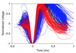
Once each cell type is identified, the main script plots all AP waveforms, while holding the same color code introduced above for narrow and broad spiking cells:
Code dependencies
The code of the waveform analysis calls plot2svg to save plots as svg files, which is available here:http://www.mathworks.com/matlabcentral/fileexchange/7401-scalable-vector-graphics–svg–export-of-figures.